Top 5 stream processing patterns for real-time data

The demand for streaming data has increased since the advent of IoT devices, mobile phones, and e-commerce. Before that, high-frequency data processing was limited to stock markets and critical systems in the airline industry. Now that both software and hardware are available to process data “on the fly”, it's essential to understand the various stream processing patterns that make real-time data processing possible.

Stream processing patterns maximize the use of the resources at your disposal. Delays in streaming data can be very costly in terms of your computing and business costs. You need to choose the correct stream processing pattern to minimize the computing power required to deliver the right results from your processing operations.

This post explains various established stream processing patterns that work across stream processing technologies, such as Apache Kafka®, Apache Flink® , and Apache Spark™.

When to use stream processing patterns

Although batch processing of data remains the most common method for reporting and analysis in businesses, an increasing number of companies are recognizing the importance of real-time data processing so they can take immediate action. Unlike batch-based processing, where incoming raw data is typically stored in a cost-effective location like Amazon S3, stream processing consumes and processes the data in its original format. This approach allows you to extract valuable insights from the data at an earlier stage.

Some of the most common use cases for stream processing include financial trading, vehicle tracking, industrial equipment sensors (IoT devices), e-commerce user analytics, fraud detection, and targeted advertising.

Take the example of vehicle tracking for any of the popular ride-hailing apps. When you take a ride, you want to ensure the driver follows the prescribed path for safety reasons. You want to be able to penalize drivers who deliberately take longer routes so that riders end up paying more. Vehicle tracking also makes tremendous business sense if you're managing a large fleet of freight trucks and want to ensure the timely delivery of goods and the safety of everyone on the truck and the road.

The finance industry has widespread real-time data processing applications, from detecting suspicious transactions to analyzing high-frequency trading. Real-time streaming analytics enabled by rolling window aggregates would allow analysts to make sense of the data and even apply algorithms to automate specific activities.

That said, let’s get into the stream processing patterns behind these applications.

5 popular stream processing patterns

Here are five stream processing patterns (in no particular order) that could power the use cases we just mentioned.

1. Filtering

Just as you can use conditions in an SQL query's WHERE clause to filter data, you can do the same with streams. Filtering removes unnecessary data elements from a stream by evaluating each element with conditions. In addition to the equality filters, you can do string matches, regex matches, range matches, and more. You can use more than one condition stringed together with a Boolean operator to apply a filter on your streaming data.

Here's a Flink SQL query for mapping a stream topic to a table. You can then query that streaming table to get the result with the users from the USA and the UK, as shown below:

CREATE TABLE users_stream (
    ts TIMESTAMP(3),
    user_name STRING,
    user_email STRING,
    user_phone STRING,
    user_country STRING,
    PRIMARY KEY (user_name, ts) NOT ENFORCED) 
  WITH (
      'connector' = 'upsert-kafka',
      'topic' = 'users',
      'properties.bootstrap.servers' = 'kafka:9094',
      'key.format' = 'json',
      'value.format' = 'json'
  );

SELECT user_name,
       user_email,
       user_phone,
       user_country
  FROM users_stream
 WHERE user_country in ('USA','UK');

Filtering in stream processing

This method frequently fetches only the data relevant to your real-time data analysis use case.

Filtering is often used with other stream processing patterns like aggregation, windowing, joining, and preprocessing, as you'll see in the following sections.

2. Stream-table joins

There are three types of joins in stream processing: stream-stream, table-table, and stream-table. With stream-stream joins, you can join two incoming data streams to create either a third stream or a table. This is very useful when you have separate systems, each with a stream of its own, and want a holistic view of your business in real time.

This article focuses on stream-table joins, which combine streaming data with materialized, physical tables. This is particularly useful for joining streaming data with reference data. Flink supports several types of joins over dynamic tables (streams). Here's a join between the dynamic table orders and a regular table products:

CREATE TABLE orders (
    order_id INT,
    quantity INT,
    order_time TIMESTAMP,
    PRIMARY KEY (order_id, order_time) NOT ENFORCED
)
WITH (
    'connector' = 'upsert-kafka',
    'topic' = 'orders',
    'properties.bootstrap.servers' = 'kafka:9094',
    'key.format' = 'json',
    'value.format' = 'json'
);

CREATE TABLE products (
    product_id INT,
    product_name INT,
    cost INT
);

SELECT p.product_id,
       p.product_name,
       SUM(o.quantity) AS products_sold,
       SUM(p.cost) AS revenue
  FROM orders o
  JOIN products p
    ON p.product_id = o.product_id
 GROUP BY p.product_id, p.product_name

Stream-table joins are also used in conjunction with the stream processing pattern that's covered later on, preprocessing. Often, streams need to look up reference data to clean and transform incoming data. In such cases, stream-table joins are used.

3. Windowing joins

A window join takes any of the join types discussed in the previous sections and adds a time window to the common key column. Windowing joins are common in stream processing because of the common use of aggregating data based on time.

For instance, consider a scenario where you have IoT sensors in a manufacturing facility that provides information about a particular motor. This motor can safely operate when its temperature is under 110 Celsius. The motor can bear momentary spikes in temperature, but if there are more than ten readings of temperature spikes per hour, it could falter and risk damaging other parts of the facility.

You want to be especially cautious about new motors installed within the last seven days, so you decide to sound an alarm when a new engine has eight readings of spikes within the first hour of its installation. Here's how you'd do it using Apache Flink SQL:

SELECT d.device_id, SUM(CASE WHEN r.reading >= 8 THEN 1 ELSE 0 END) spike_count
 FROM readings r, devices d
WHERE r.device_id = d.device_id
  AND r.reading_time BETWEEN d.installation_time AND u.installation_time + INTERVAL '1' HOUR
  AND d.installation_time BETWEEN CURRENT_TIMESTAMP() - INTERVAL '7' DAY AND CURRENT_TIMESTAMP()
GROUP BY d.device_id;

4. Preprocessing

Preprocessing is also known as the transformation pattern and is one of the most critical processing patterns in streaming. Preprocessing makes streaming data ready to be used for further querying and analysis. This pattern can involve record transformation at an event level, such as exploding a nested JSON, or at a field level, such as breaking the value of a key in the JSON structure into two.

For instance, imagine a scenario where you have three types of temperature sensors installed in different manufacturing facilities. These IoT devices might operate with different standards and send events in different formats. In such cases, you'd want to standardize/normalize your incoming data as early as possible to avoid downstream processing. Here's an example where a user's activity is pictured in a JSON field, from which individual fields are extracted as separate columns:

SELECT 
 user_id,
 SPLIT_INDEX(user_name, ' ', 0) first_name,
 SPLIT_INDEX(user_name, ' ', 1) last_name,
 JSON_VALUE(activity_detail, '$.type') activity_type,
 JSON_VALUE(activity_detail, '$.duration') activity_duration,
 TO_TIMESTAMP(FROM_UNIXTIME(JSON_VALUE(activity_detail, '$.starttime'))) activity_start_time,
 TO_TIMESTAMP(FROM_UNIXTIME(JSON_VALUE(activity_detail, '$.endtime'))) activity_end_time,
FROM user_activity;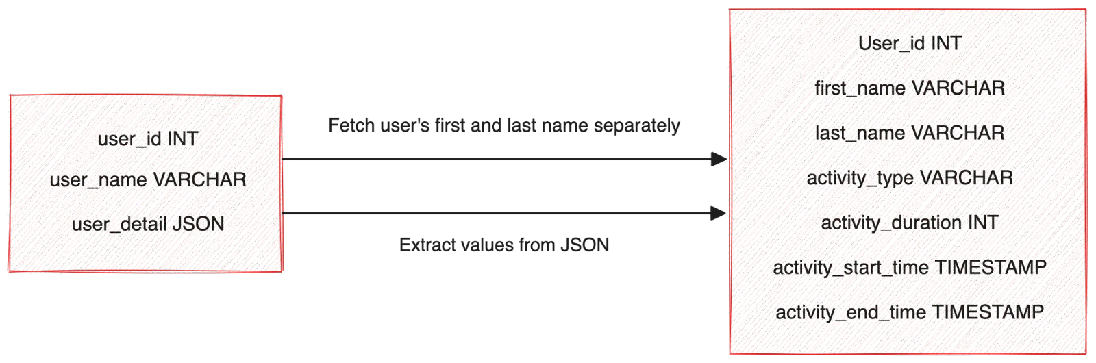

Preprocessing and transformation in stream processing

This initial processing and transformation of streaming data also prevents the undue load of performing these transformations downstream.

5. Aggregation

Stream processing often uses a particular type of aggregation pattern called windowed aggregation. This pattern is popular because, in most cases, you'd need to look at the most recent data in a streaming application based on a business rule or condition.

For instance, you might want to look at the sum of sales in the last hour or the average sale amount based on the previous hundred sale orders. There are many ways of aggregating streaming data:

• Hopping window aggregation: A hopping window is defined by a set time window but moving start and end times.
• Tumbling window aggregation: A tumbling window is a case of hopping window aggregation where both the time window and the advance window are defined and of equal sizes, meaning that an event will only ever land up in one window and not more.
• Session window aggregation: A session window is defined by the idle time between two activities. This gap between the two activities is called the inactivity gap.

The following image shows how hopping and tumbling windows differ:

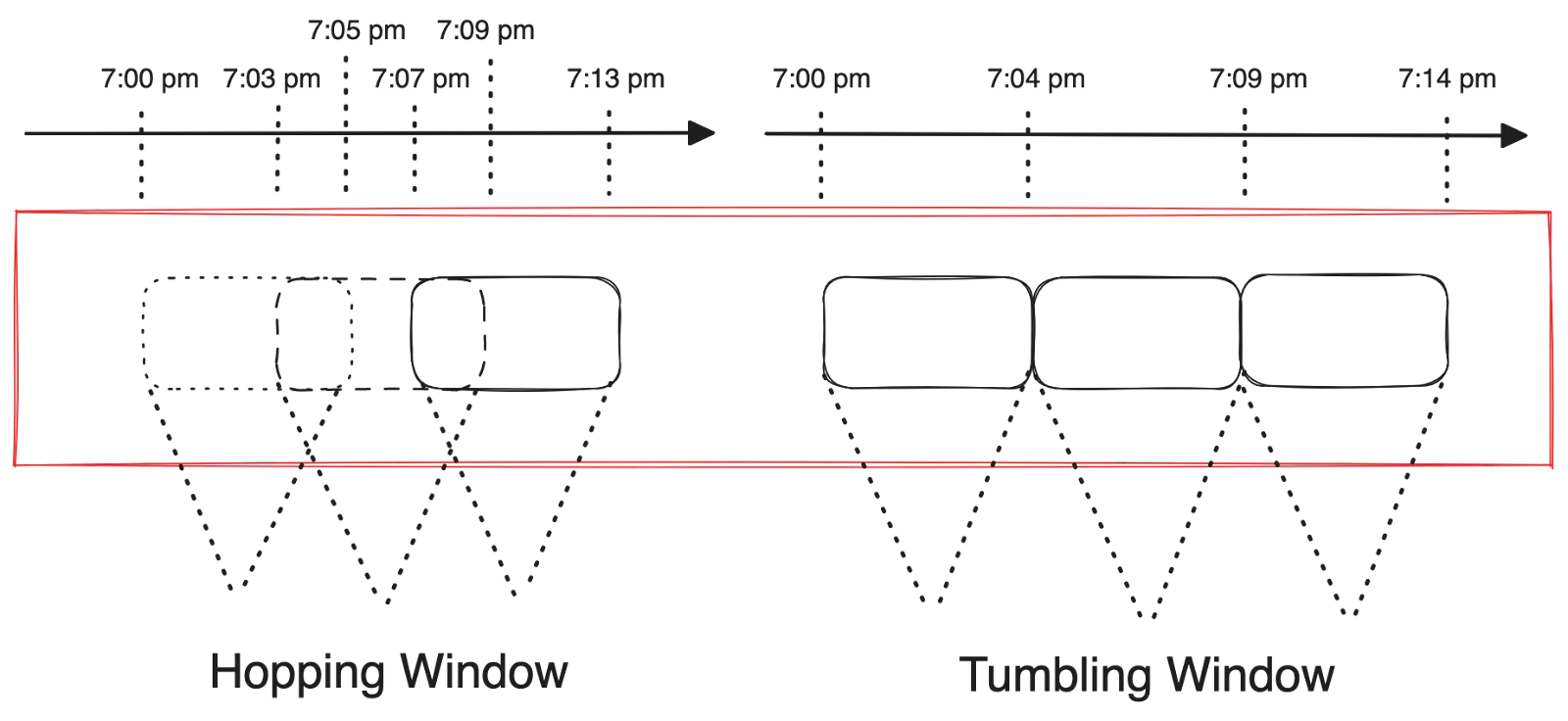
Hopping windows and tumbling windows

The following example shows how you can write a query to aggregate the number of user activities based on specific regions for every five-minute tumbling window in Flink SQL:

SELECT window_start, 
       window_end,
       activity_region,
       COUNT(*) AS cnt
  FROM TABLE(TUMBLE(TABLE user_activity, DESCRIPTOR(user_activity_time), INTERVAL '5' MINUTES))
 WHERE LCASE(user_activity_type) IN ('add_to_cart','order_placed')
 GROUP BY window_start, window_end, activity_region;

There are many other special cases of windows, such as cumulative windows and sliding windows, but they are specific to different stream processing engines.

Conclusion

This post explored some of the most popular stream processing patterns, such as filtering, window joins, preprocessing (transformation), and aggregations. If you'd like to delve further into this topic, you can explore various other less common stream processing patterns, such as the machine learning (ML) pattern or the sequential convoy pattern.

Stream processing is an everyday use case for many businesses, as they want to consume insights as early as possible. Redpanda is a streaming data platform compatible with the Kafka API that eliminates all the complexity of Kafka's underlying technologies. Redpanda has taken a fresh approach to making streaming data fast and reliable.

To get started with Redpanda for simpler real-time streaming, check the documentation and browse the Redpanda blog for tutorials. To chat with the team and fellow Redpanda users, join the Redpanda Community on Slack!