Real-time ML analysis with TensorFlow, BigQuery, and Redpanda

Real-time data processing is gaining popularity due to the immense volume of data generated. When machine learning is applied to real-time data for instantaneous results and low latency, it's referred to as "real-time machine learning analysis." Unlike traditional machine learning models, real-time ML models are actively involved in making predictions and they update or retrain themselves on this new data as it comes in to make accurate predictions.

In this post, you'll learn about real-time machine learning and a few popular use cases like real-time fraud detection, real-time chat systems, virtual health assistants, and e-commerce recommendation systems. To wrap it up, we’ll walk you through how to implement a real-time ML analysis system for fraud detection using TensorFlow, BigQuery, and Redpanda.

Understanding machine learning and real-time ML analysis

In traditional programming, you define all the steps and logic to perform a task based on the data provided. ML, on the other hand, relies on training a computer using large data sets, allowing it to identify patterns and relationships autonomously. The core process of ML involves:

• Data collection
• Data processing
• Feature selection
• Model selection
• Model training and evaluation
• Model deployment

Real-time ML analysis prioritizes low latency and adaptability, enabling models to update parameters as new real-time data arrives without the need for batch processing. Such systems require vast data volumes while maintaining performance.

Machine learning has a wide variety of use cases in real-time applications. Real-time fraud detection employs forensic analytics and predictive analytics to swiftly identify credit card and financial payment fraud, ensuring prompt responses while protecting legitimate transactions. Real-time chat systems employ natural language processing (NLP) algorithms and large language models (LLMs) to respond to user queries instantly.

Tools like ChatGPT and Google Bard are transforming how user queries are addressed in general. In healthcare, ML-powered virtual assistant systems provide timely healthcare feedback, enhancing health insights and reducing employee fatigue in healthcare institutions.

Furthermore, in e-commerce, real-time analytics improve recommendation systems by swiftly updating models with current user data, delivering immediate and valuable insights for personalized item or service recommendations.

How to build real-time ML analysis with TensorFlow, BigQuery, and Redpanda

In this tutorial, you'll use TensorFlow, BigQuery, and Redpanda to implement a real-time credit card fraud detection system.

TensorFlow is a widely used framework for large-scale machine learning and numerical computations, offering various ML algorithms and neural network implementations. BigQuery, part of the Google Cloud Platform, is a serverless, cost-effective multicloud data warehouse. It enables the storage and querying of extensive data sets without infrastructure management, and it utilizes columnar storage for improved query speed.

However, while BigQuery excels at storing real-time data, it doesn't directly manage event data from streaming platforms. This is where Redpanda comes in. It seamlessly integrates with BigQuery and enables real-time streaming and writing of data into BigQuery tables.

The application you'll build will read and write real-time data into BigQuery, use a TensorFlow CNN-based classification model, and use Redpanda to stream structured data in real time:

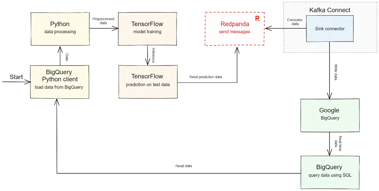
Solution architecture diagram for real-time fraud detection

The example data set you'll use is a popular credit card fraud detection data set from Kaggle. This data set contains values that are already preprocessed, so you don't need to perform much data preprocessing. The data set has been divided into training and testing sets and can be downloaded here.

Prerequisites

This post assumes that you have Redpanda and Kafka Connect already set up. If not, follow this tutorial.

Note: While setting up Redpanda on macOS, you may get an error stating that "request size is larger than configured size" with Kafka configuration. Using

--set redpanda.kafka_batch_max_bytes=2097152000
--set redpanda.kafka_request_max_bytes=2097152000

as the Docker parameters while building the image should resolve the issue.

You'll also need the following:

• A macOS environment with the Homebrew package manager
• The latest version of Docker Desktop and a running instance of Redpanda
• The Python programming language (any version higher than 3.10) and Jupyter Notebook for writing interactive code
• The latest version of the TensorFlow library installed as a Python package
• A Google Cloud Platform (GCP) free tier account for BigQuery
• A local folder with the name pandaq_integration (as shown here), where you'll store data related to the project

Setting up BigQuery

To set up BigQuery for your use case, open your BigQuery dashboard and check the dropdown menu in the upper left corner. This option shows the currently selected project. If there are no projects to choose from, you need to create one by clicking the NEW PROJECT button.

For example, a project with the name redpandaq would look like this:

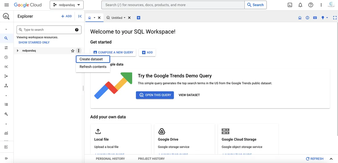
This particular project is selected by default as there is no other project in the menu. If you have multiple options, you can choose any one to proceed with. Once you select a project, you need to create a data set for your fraud classification use case.

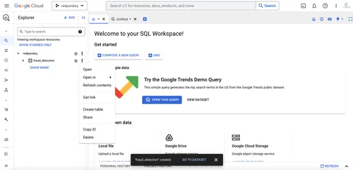
Click the three dots next to the project name in the left panel and select the Create dataset option:

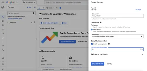
Provide the required details and click CREATE DATASET:

Click the three dots next to your created data set to create a table for storing your training data:

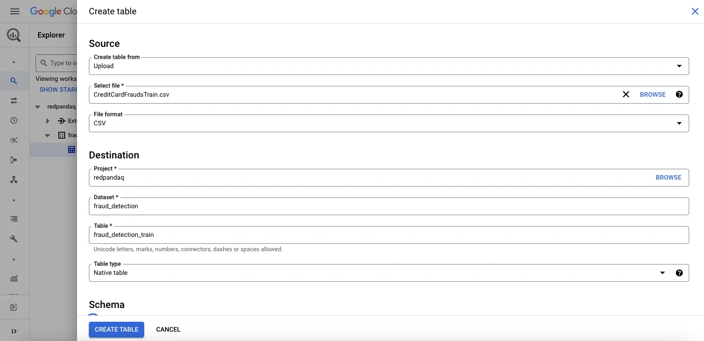
In the form that opens, select Upload under the Create table from field, then browse for and select the local file for the data set. Provide the table name, set automatic schema creation, and click CREATE TABLE:

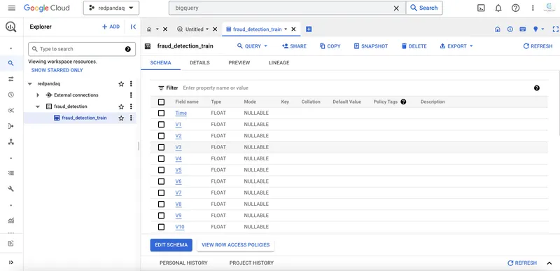
Once you create the table with the fraud detection data, you can click the data set in the Explorer section to check out different details of the uploaded data:

Next, you'll set up a GCP service account to access this data using the Python client or with Redpanda.

Setting up a GCP service account

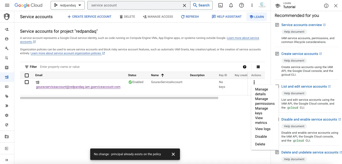
In the top search bar, search for "service account" and click the Service Accounts link.

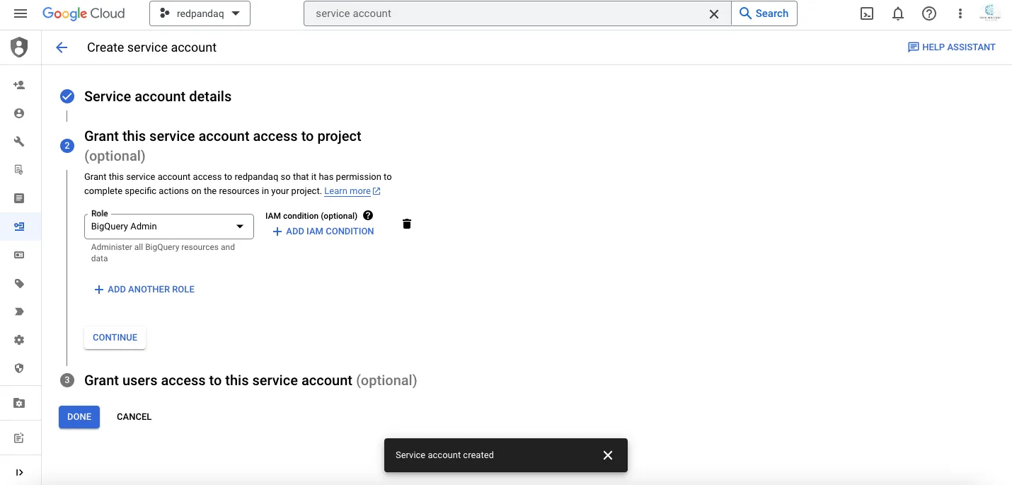
On the new page that opens, click the CREATE SERVICE ACCOUNT button. Provide a service name (such as bigquery-account) and click CREATE AND CONTINUE. You also need to select a role for this service account. An admin role typically has full access to any service. To assign an admin role, select the BigQuery Admin role and click CONTINUE:

On the next page, click the three dots and choose the Manage keys option:

Next, click the Add Key button and then select the Create New Key option. Save the resulting credentials JSON file and keep it safe, as you'll need it for further configuration.

Training the fraud detection model using TensorFlow

With the initial set up complete, you now need to train your fraud detection model using TensorFlow.

Loading dependencies

Start Jupyter Notebook and create a new notebook with the name Fraud-Detection-with-TensorFlow-and-BigQuery. Within this notebook, you'll import all the necessary Python dependencies for reading data, preprocessing, modeling, and charting.

All these libraries can be installed with the help of pip:

$ pip install google-cloud-bigquery
$ pip install db-types
$ pip install pandas numpy matplotlib
$ pip install imblearn
$ pip install sklearn
$ pip install tensorflow

Once they're installed, you can load these libraries as follows:

# Google BigQuery dependencies
from google.cloud import bigquery
from google.oauth2 import service_account

# Load and store pickle objects
import pickle

# Mathematical computations and DataFrame manipulation
import numpy as np
import pandas as pd
from numpy import asarray

# Data sampling 
import imblearn
from imblearn.over_sampling import SMOTE

# Plotting and visualization
import matplotlib.pyplot as plt

# Model data preprocessing
from sklearn.model_selection import train_test_split
from sklearn.preprocessing import StandardScaler

# Modeling
import tensorflow as tf
from tensorflow import keras
from tensorflow.keras import Sequential
from tensorflow.keras.layers import Flatten, Dense, Dropout, BatchNormalization
from tensorflow.keras.layers import Conv1D, MaxPool1D
from tensorflow.keras.optimizers import Adam

Reading data from BigQuery using a Python client

You'll next create a BigQuery Python client that will interact with BigQuery to read and write data. You'll need the credentials JSON file that you downloaded earlier.

Call the bigquery.Client() function by providing the credentials file and the project name as follows:

# Define BigQuery credentials
credentials = service_account.Credentials.from_service_account_file('/path-to/gcp-redpandaq-admin.json')
project_id = 'redpandaq'

# Initiate BigQuery client
client = bigquery.Client(credentials= credentials,project=project_id)

Once you run the above code, you'll be connected to the BigQuery instance, letting you query data from the BigQuery data set using simple SQL syntax as follows:

# Query data from BigQuery
query_job = client.query("""SELECT *
                        	FROM fraud_detection.fraud_detection_train""")

results = query_job.result()

You need to process a structured tabular data set, and the commonly employed tool for this purpose is pandas.DataFrame(). Convert the queried data into a DataFrame using the to_dataframe() function:

# Convert to DataFrame
data = results.to_dataframe()
# Check first few rows of the data
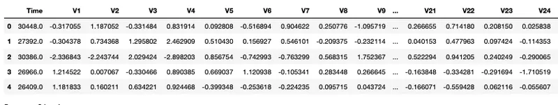
data.head()

Your queried data set should look something like this:

Applying data quality checks

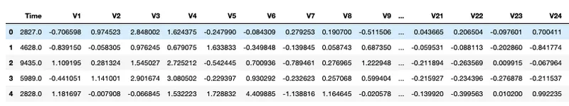
Once the data is loaded from BigQuery, you need to apply some quality checks before proceeding with modeling. Start by checking the null values in the data set:

# Check null values
data.isnull().sum()

You also have the option to examine more comprehensive details about the data using the info() method from pandas, which provides insights like non-null columns, data types, memory usage, and more:

# Check DataFrame information
data.info()

One of the most important things for any real-world classification use case is verifying the ratio of the classes you want to predict:

# Check class count
data['Class'].value_counts()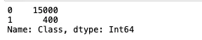

The number of fraudulent cases in the data set is much lower than the non-fraudulent ones, which results in a data imbalance problem. This imbalance affects the model's performance because the results produced by the model will always be biased toward the majority class. You'll resolve this issue a bit later.

TensorFlow also requires model inputs and outputs to be float, so make sure all your column values are float. If they're not, you can convert them using the astype() method:

# Convert class column to float
data['Class'] = data['Class'].astype('float64')
data.info()

Splitting Data into Training and Validation Sets

Although the data is already divided into training and testing sets, you need to create one more partition from the training set called the validation set. The model uses this data set to validate its results and adjust the neural network weights accordingly.

To create this partition, first create two different variables for input and output:

# Separate input and output values
X_values = data.drop('Class', axis = 1)
y_values = data['Class']

Then, use the train_test_split() method from sklearn.model_selection to split the data into training and validation sets. Make sure to stratify this data set on the output value for better distribution based on class:

# Split data into train and test sets
X_train, X_test, y_train, y_test = train_test_split(X_values, y_values, test_size = 0.2, random_state = 0, stratify = y_values)

# Check shape of data
X_train.shape, X_test.shape

Addressing Data Imbalance Using SMOTE Oversampling

Once you have the training and validation sets, you need to work on the class imbalance problem. Otherwise, the results that the model produces will be biased toward the majority class.

There are multiple ways to handle the class imbalance problem. For this use case, you'll use the SMOTE oversampling method to generate the minority samples and bring them up to the level of the majority samples:

# Apply SMOTE oversampling
oversample = SMOTE()
X_train, y_train = oversample.fit_resample(X_train, y_train)

Once SMOTE is applied, the distribution of the data set will change. You can check the new distribution with the following code:

# Summarize the new class distribution
from collections import Counter
counter = Counter(y_train)
print(counter)

Data scaling

When you look at the data, you might find that different columns have values at different scales. So, you need to standardize your data using a scaling mechanism. You can use standard scaling to do this.

The sklearn library provides an implementation of standard scaling with the StandardScaler() function:

# Create object of standard scaler
scaler = StandardScaler()
X_train = scaler.fit_transform(X_train)
X_test = scaler.transform(X_test)

# Convert data to numpy arrays
y_train = y_train.to_numpy()
y_test = y_test.to_numpy()

# Save the scaler for future use
with open('data/StandardScaler.pkl','wb') as f:
	pickle.dump(scaler, f)

Make sure you save the standard scaler in a pickle file because the same scaling configurations might be used in production to make the predictions for the real-time data (test data in this case).

The final step before ML modeling is converting your 2D data to 3D, which is a requirement for the TensorFlow-based models.

This can be done with the help of the reshape() method from numpy:

# Convert data to 3D
X_train = X_train.reshape(X_train.shape[0], X_train.shape[1], 1)
X_test = X_test.reshape(X_test.shape[0], X_test.shape[1], 1)

# Check shape of data
X_train.shape, X_test.shape

Training and saving the deep learning model

Now that your data is ready, you can use TensorFlow to create a CNN architecture. This architecture will be made up of two convolution 1D layers with batch normalization and an added dropout rate of 50 percent, one flattening layer with batch normalization and an added dropout rate of 50 percent, and a dense layer for classification.

As you need these layers in sequence, you'll use the Sequential() method from TensorFlow and add all these layers using the model.add() method:

# Define model architecture
epochs = 10
model = Sequential()

model.add(Conv1D(32, 2, activation='relu', input_shape = X_train[0].shape))
model.add(BatchNormalization())
model.add(Dropout(0.2))

model.add(Conv1D(64, 2, activation='relu'))
model.add(BatchNormalization())
model.add(Dropout(0.5))

model.add(Flatten())
model.add(Dense(64, activation='relu'))
model.add(Dropout(0.5))

model.add(Dense(1, activation='sigmoid'))
model.summary()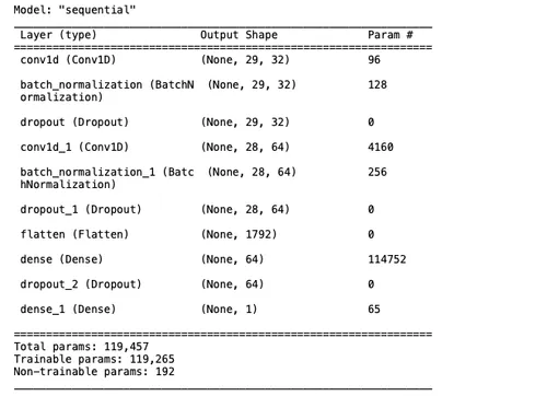

To train this model, you'll use Adam optimization (preferred for CNN). The loss function employed will be binary_crossentropy, as this is a binary classification problem. Furthermore, now that the data set is more balanced, the selected metric will be accuracy. You'll train the model for ten epochs and validate the model's performance on the provided validation data:

# Train model
model.compile(optimizer=Adam(lr=0.0001), loss = 'binary_crossentropy', metrics=['accuracy'])
history = model.fit(X_train, y_train, epochs=epochs, validation_data=(X_test, y_test), verbose=1)

As you can observe in the above image, only three epochs would have been enough to get the best accuracy from the model. This will change depending on the type of data and the number of layers you are using for your use case. Finally, you need to save the model architecture and weights to use them for the test data. This can be done using the save() method as follows:

# Save model architecture and weights
model.save("data/fraud_detection_model.h5")

Testing the fraud detection model

Create one more notebook named Real-Time-Fraud-Detection-with-TensorFlow-BigQuery-and-Redpanda.ipynb, which you'll use to make predictions for the test data, and send it over to BigQuery using Redpanda.

Import the required dependencies for model inference:

# Load dependencies
import pickle
import pandas as pd
from tensorflow.keras.models import load_model

Load the testing data set to make a prediction using the trained CNN model:

# Read CSV data set
data = pd.read_csv('data/CreditCardFraudsTest.csv')
data.head()

The testing data set should look something like this:

Once the data is loaded, you need to load the standard scaler configurations that you stored at the time of training. This is because you want to apply the same preprocessing steps to the testing data as you did with training:

# Load standard scaler from pickle
with open('data/StandardScaler.pkl','rb') as f:
	scaler = pickle.load(f)

# Apply standard scaling on the data
data_test = scaler.fit_transform(data_test)

Use the following code to convert this data to 3D for the TensorFlow model:

# Reshape data to 3D for prediction
data_test = data_test.reshape(data_test.shape[0], data_test.shape[1], 1)
data_test.shape

Finally, load the trained model for making the prediction:

# Load model
model = load_model('data/fraud_detection_model.h5')
model.summary()

Call the predict() method on this data. This method produces the results in float values that are hard to interpret, so you need to convert the results to int to read them as binary values:

# Make predictions
predictions = model.predict(data_test)
# Convert predictions to binary
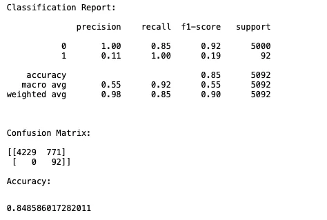
predictions = predictions.astype(int)

You can use the sklearn.metrics module to view different metrics like precision, recall, and accuracy and check the performance of the model on the testing data:

# Check model performance
from sklearn.metrics import classification_report, confusion_matrix, accuracy_score
print('Classification Report:\n')
print(classification_report(data['Class'], predictions), '\n')
print('\nConfusion Matrix:\n')
print(confusion_matrix(data['Class'], predictions))
print('\nAccuracy:\n')
accuracy_score(data['Class'], predictions)

The model's performance should look something like this:

You now need to store the predicted data in JSON format in the pandaq_integration folder that you created during Redpanda and Kafka setup. You'll stream the data in the JSON file to BigQuery with the help of Redpanda.

To do so, assign the predicted values to the Class volume as follows:

# Create predictions column in original DataFrame
data['Class'] = predictions

# Check first few rows
data.head()

Note: To avoid an error, make sure that your streaming data has the same schema as the data stored in BigQuery.

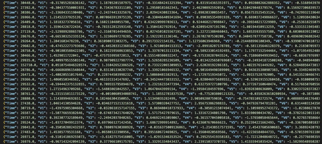
To store the data as JSON, you need to first convert the final DataFrame into a dictionary using the to_dict() method, then use the csv_jsonl library to convert this dictionary to JSON and store it in the pandaq_integration folder:

# Convert data to dict
data_to_dict = data.to_dict(orient = 'records')

# JSON file path
jsonFilePath = '/Home/pandaq_integration/fraud_detection_predictions.json'

# Store data in JSON
from csv_jsonl import JSONLinesDictWriter
with open(jsonFilePath, "w", encoding="utf-8") as _fh:
	writer = JSONLinesDictWriter(_fh)
	writer.writerows(data_to_dict)

The resultant data might look something like this:

Sending Messages to BigQuery Using Redpanda

Finally, you'll stream the data to BigQuery using Redpanda. This section assumes that the Redpanda Docker image is already running on localhost:9092. To begin streaming, you need to create a Redpanda topic with the same name as your BigQuery data set. That's fraud_detection_train in this case:

$ docker exec -it redpanda-1 \
rpk topic create fraud_detection_train

redpanda-1 is the container image name. Make sure you use your container image's name if it differs.

You can check the cluster info with the help of the following command:

$ docker exec -it redpanda-1 \
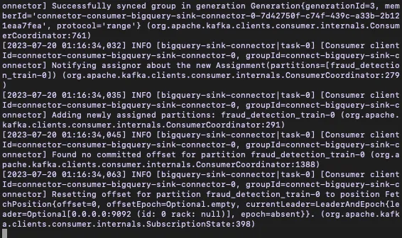
rpk cluster info

Run the Kafka Connect script inside the pandaq_integration/configuration folder as follows:

$ ../kafka_2.13-3.1.0/bin/connect-standalone.sh connect.properties bigquery-sink-connector.properties

$ ../kafka_2.13-3.1.0/bin/connect-standalone.sh connect.properties bigquery-sink-connector.properties

You should see an output like this:

Finally, to send the data to BigQuery using Redpanda, run the following command, providing the topic name and path to the JSON file:

$ docker exec -it redpanda-1 /bin/sh -c \
'rpk topic produce fraud_detection_train < /tmp/pandaq_integration/fraud_detection_predictions.json'

You should see an output similar to the following:

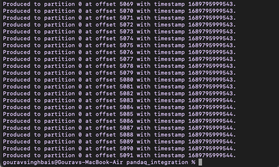
If you face any issues related to the file not being found, make sure that the local pandaq_integration folder is correctly mapped to the Redpanda image when building the Docker image.

Once you run the above command, the number of records present in your JSON file will be sent to the BigQuery data set. You can verify this result by going to your BigQuery account and clicking the fraud_detection_train table, then clicking Query > In new tab to open the query console. Run the SQL query to select the data from the table. You will be able to see the recently streamed rows in the data set:

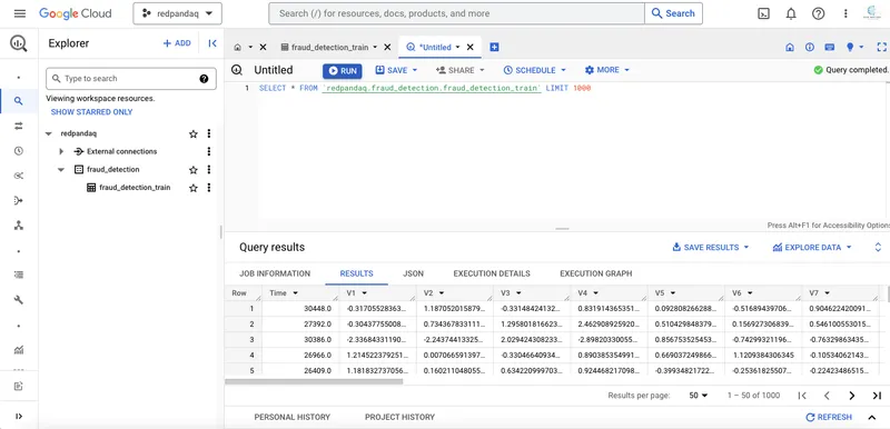
You can now cross-check the data in BigQuery with the information stored in your JSON file; they should match.

That's it! You've successfully created a fraud detection system with the help of BigQuery, TensorFlow, and Repanda. Although there is much more to the field of real-time machine learning, this is a good starting point.

Conclusion

This post introduced you to real-time machine learning and its various use cases. You also learned how to create a real-time fraud detection system using TensorFlow and BigQuery! Most important of all, you now know how to read messages from Redpanda and send them to BigQuery using Kafka Connect, after which you can execute SQL queries on BigQuery to analyze your data.

You can find all the resources used to create the real-time fraud detection system in this GitHub repository. To keep exploring Redpanda, check the documentation and browse the Redpanda blog for tutorials. If you have any questions or just want to chat with the team and fellow Redpanda users, join the Redpanda community on Slack.

Machine learning (ML) involves creating algorithms and mathematical models that empower computers to learn and enhance their performance for tasks like prediction and pattern recognition. These algorithms learn from historical data and use this knowledge to predict outcomes for new data.