

Data lifecycle management—Stages, patterns, and technologies


Data lifecycle management
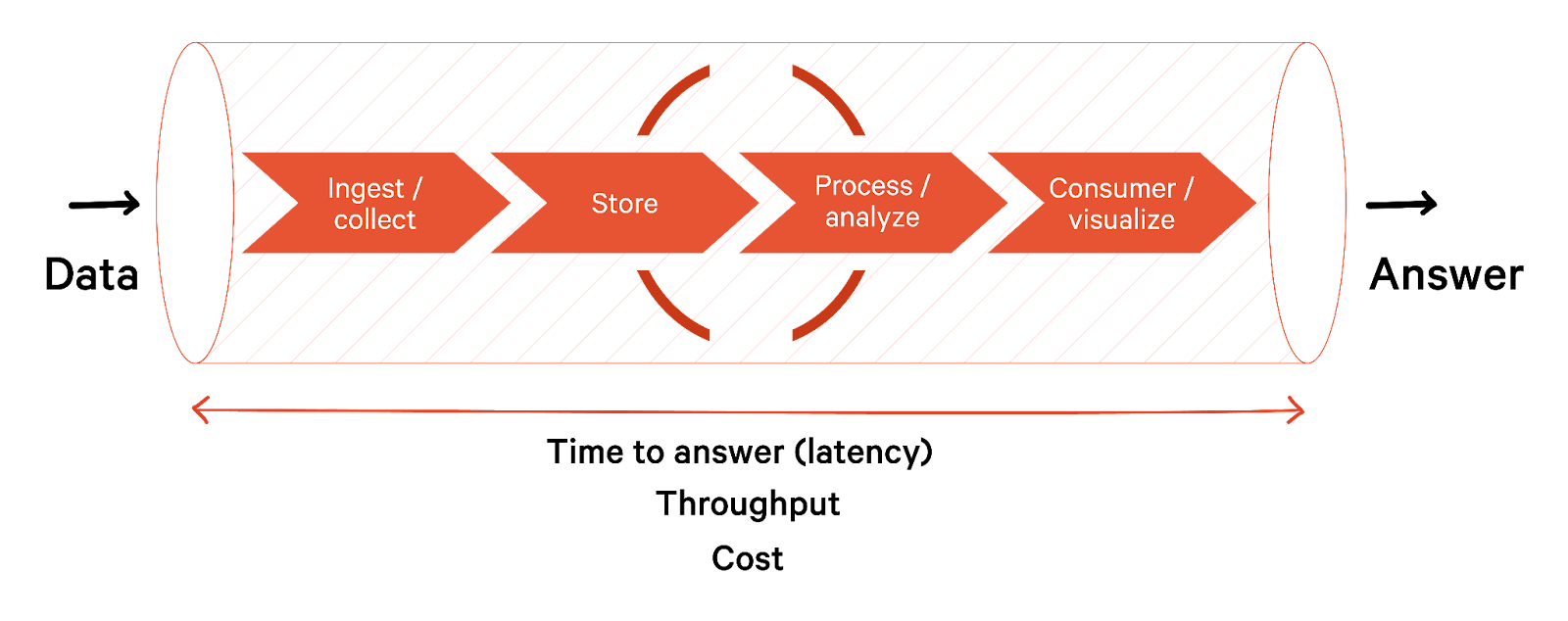
Data lifecycle management (DLM) is the process of managing your data, from creation and collection to storage and transformation, consumption, and final deletion or archival. DLM aims to ensure that data is accurate, complete, and easily accessible to its users. Steps are taken at every stage to protect data from unauthorized access, corruption, or loss.
This article thoroughly explores data lifecycle management stages, including patterns and technologies. We also look at some data lifecycle management best practices for improved efficiency.
Summary of data lifecycle management stages
We summarize the data lifecycle management stages that provide a framework for working with data below.
| Phase | Description |
|---|---|
| Data generation | The process of creating new data, either by collecting it from various sources or by generating it through algorithms and models. |
| Data ingestion | Collect and transport data from various sources, such as databases, APIs, and files. |
| Data storage | Store data in a scalable and reliable manner, such as in data warehouses, data lakes, or databases. |
| Data processing & transformation | Process data to make it suitable for analysis, such as data integration, cleansing, and quality checks. |
| Data consumption | Involves data analysis to extract insights, create reports and dashboards to visualize data and distribute data to various stakeholders. |
| Data retention | Develop policies and procedures for retaining data for a specific period based on legal or business requirements. |
| Data archiving | Long-term storage for data that is no longer needed for immediate analysis or reporting but may be needed in the future. |
| Data deletion | Delete data that is no longer required based on legal or business requirements. |
Data generation
Data generation source systems in big data engineering produce or collect data that can be used for analysis or other purposes. Some standard data generation source systems include:
- IoT systems that collect data from various sources, such as sensors, cameras, and GPS devices.
- Mobile apps that generate data related to user behavior, such as app usage, user demographics, and location tracking.
- Application, server, and system logs that collect data about system health and behavior that are valuable for downstream data analysis, ML, and automation.
- Message queues and event streams that collect event data as messages.
Apart from the above, human-generated information like application forms, transactions, surveys, and polls comprise a large portion of data.
Data ingestion
There are several techniques used for data ingestion, depending on the data source, the data volume, and the desired outcome. In the push model of data ingestion, a source system writes data out to a target, whether a database, object store or filesystem.
In the pull model, data is retrieved from the source system. The line between the push and pull paradigms can be quite blurry; data is often pushed and pulled as it works through various stages of a data pipeline.
Extract, Transform, Load (ETL) is a traditional data integration technique that involves extracting data from various sources, transforming it into a standard format, and loading it into a target system such as a data warehouse or data lake. ETL evolved further into Extract, Load, Transform (ELT), which extracts data from various sources, loads it into a centralized repository, and transforms it into a format that is optimized for analysis and processing.
However, both ETL and ELT present challenges at scale. Transforming data from different sources and formats into a common format for analysis is time and resource-intensive. In such cases, we use data federation, which allows data to be accessed and consumed across multiple systems without physically moving the data. It uses virtualization layers to create a unified data view across different systems.
Data ingestion patterns
Ingestion patterns describe solutions to commonly encountered problems in the data source to ingestion layer communications.
- Multisource extractor pattern is an approach to ingest multiple data source types efficiently.
- Protocol converter pattern employs a protocol mediator to provide the abstraction for the incoming data from the different protocol layers.
- Multidestination pattern is useful when the ingestion layer has to transport the data to multiple components like Hadoop Distributed File System (HDFS), streaming pipelines, or real-time processing engines.
- Just-in-time transformation pattern involves transforming data into a format suitable for consumption by the target system just before it is needed to save compute time.
- Real-time streaming patterns support instant analysis of data coming into the enterprise
[CTA_MODULE]
Data storage
Now that we have looked into how data is generated and ingested, let's look into the different storage options in data lifecycle management. Initially, data was primarily stored in databases. As data use cases changed, other storage architectures like warehouse and lake emerged.
Databases
Relational databases like MySQL, PostgreSQL, and MariaDB store data in a structured format, using tables and rows to organize and manage data. You define the data schema before writing the data to the database (schema on write).
In contrast, NoSQL databases handle large amounts of unstructured and semi-structured data that cannot fit well into tabular formats. They allow you to define the data schema only at access time (schema on read) for more flexibility and scalability. Some NoSQL databases include:
| NoSQL Database Type | Description | Technology |
|---|---|---|
| Key-value store | Associate data values with keys. | Redis, Memcached, and Ehcache. |
| Column store | Store multiple key (column) and value pairs in each row. You can write any number of columns during the write phase and specify only the columns you are interested in processing during retrieval. | Apache Cassandra, Apache HBase |
| Document store | Store semi-structured data such as JSON and XML documents. | MongoDB, Apache CouchDB, and CouchBase |
| Graph store | Store data as nodes and use edges to represent the relationship between data nodes. | Neo4j |
Other data storage architectures
A data warehouse stores structured and curated data in a relational database or a cloud service. They use a predefined schema and a dimensional model to organize the data into facts and dimensions. Some of the best data warehouse tools are:
- Google BigQuery
- Amazon Redshift
- Snowflake
- Vertica
A data lake stores raw and unstructured data in a centralized repository, usually on a cloud platform or a distributed file system. It allows you to ingest data from various sources and formats without imposing schema or structure. For example, Amazon S3, Azure Data Lake, and Google Cloud Storage can be options in cloud offerings, and HDFS (Hadoop Distributed File System) is an on-premise option.
A data hub is a pattern that acts as a central mediation point between various data sources and data consumers. It is an architectural approach that integrates data from various sources using different layers and zones to separate the data by quality, purpose, and access. It can then act as a gateway to multiple consumers. The hub does not store data directly but may act as one for consumers. Here are a few examples:
- Google Ads
- Cloudera Enterprise
- Cumulocity IoT
A data lakehouse, a centralized repository that stores raw, unprocessed data in its native format, without any predefined schema. The idea behind a data lakehouse is to have a single source of truth for all data, where data from various sources can be stored, processed, and analyzed in a scalable and flexible manner.
In our chapter on data warehouse vs. data lake, we cover the above data storage architectures in more detail.
[CTA_MODULE]
Data processing & transformations
This stage of data lifecycle management focuses on preparing raw data so it is useful for analytics. There are two main categories of data processing.
Real time data processing
It is the analyzing of large volumes of data in real-time, or near-time, as it is generated or received from various sources. It allows for immediate insights and decision-making and the ability to react to changes in the data in real-time. Some technologies used include:
- Apache Storm
- Apache Flink
- Apache Spark Streaming
- Apache Kafka Streams
- AWS Kinesis
- Azure Stream Analytics
Streaming transformations are a way to process data in real-time without having to store it in a file or database first. This is particularly useful when dealing with large datasets that cannot fit into memory or when data is constantly generated at such a high rate that traditional batch processing cannot keep up.
Several patterns can be used when working with streaming transformations, including:
Windowing
The stream processor groups events together into windows based on some criteria, such as a user ID or a timestamp range. The processor then processes each window independently, allowing for more efficient processing of related events.
Triggering
The stream processor waits for a specific event or set of events to occur before triggering a processing job. This can be useful when processing data that has a low rate of change but requires immediate processing when certain conditions are met.
Late arrival handling
The stream processor handles late-arriving events by either discarding them or processing them separately from the main stream. This is useful when dealing with streams where events may arrive out of order or with delays.
Stateful processing
The stream processor maintains state across multiple events, allowing it to perform complex event processing and aggregation. This can be useful when processing data that contains periodic or aggregate information.
Real-time join
The stream processor performs real-time joins between two or more streams, allowing for the combination of data from different sources in real-time.
Real-time aggregation
The stream processor performs real-time data aggregation, such as calculating statistics or counting the number of events.
Real-time filtering
The stream processor filters out unwanted events in real-time, allowing for a reduced volume of data to be processed.
Route pattern
Route pattern is a streaming transformation pattern that involves routing incoming data streams to different branches based on certain criteria. This pattern is commonly used in big data processing applications where data needs to be processed differently depending on its characteristics, such as source, format, or content.
Transform
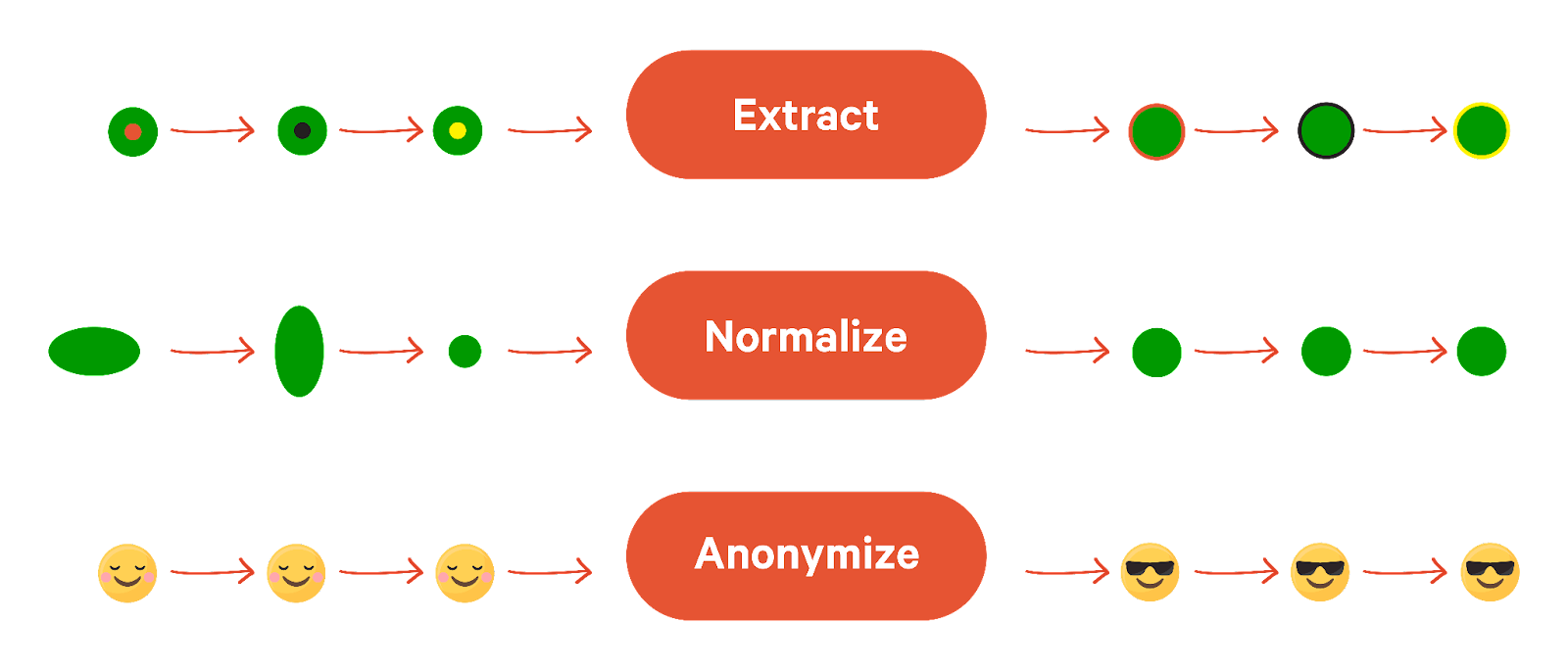
Transform involves applying a set of transformations to an input stream to produce an output stream. This pattern is commonly used in big data processing applications where data must be transformed or aggregated in real-time before being written to a destination. Different transformations include:
- Extract specific fields or values from the input data, such as extracting a customer ID from a customer record.
- Normalize the input data, such as converting all date fields to a standard format.
- Anonymize the input data, such as removing personally identifiable information (PII) from a dataset.
Windowing
The stream processor divides the input stream into fixed or variable-sized windows, processes each window independently, and then moves on to the next window. This allows for efficient processing of large datasets while still maintaining a level of parallelism. There are two types of window operations.
Keyed Windows allow for the grouping of data streams based on a specific key. Let’s take a look at the code snippet on how to do this using Flink:
Non-keyed windows are a type of window that does not require a key to be specified for grouping and aggregating data. See the Flink code snippet below.
Batch-based data processing
In batch-based data processing, data is collected over time and stored in a buffer or queue. Once the buffer is full or a specific time interval has been reached, the data is processed in a batch. Some technologies used include Apache Hadoop, MapReduce, Spark, Storm, and Flink.
Batch transformations run on discrete chunks of data. Common batch transformation patterns are given below.
MapReduce
A simple MapReduce job consists of a collection of map tasks that read individual data blocks scattered across the nodes, followed by a shuffle that redistributes result data across the cluster and a reduce step that aggregates data on each node.
Distributed joins
Distributed joins break a logical join (the join defined by the query logic) into much smaller node joins that run on individual servers in the cluster.
Broadcast join
A broadcast join is generally asymmetric, with one large table distributed across nodes and one small table that can easily fit on a single node. The query engine “broadcasts” the small table (table A) out to all nodes, where it gets joined to the parts of the large table (table B).
Sort merge join
It is an optimization technique used in database systems to improve the performance of joins between two large tables. It works by first sorting both tables and then merging them together, rather than performing a full cross-product join.
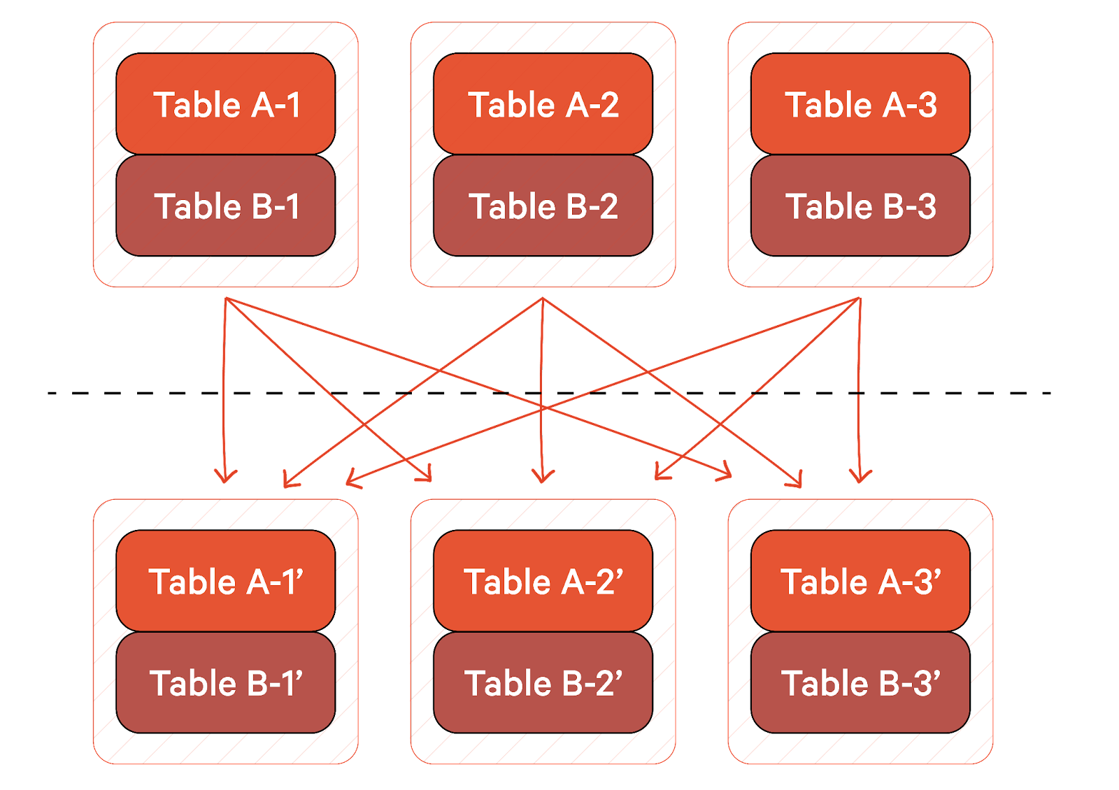
Shuffle hash join
If neither table is small enough to fit on a single node, the query engine will use a shuffle hash join. In the below figure, the same nodes are represented above and below the dotted line. The area above the dotted line represents the initial partitioning of tables A and B across the nodes. A hashing scheme is used to repartition data by join key. The hashing scheme will partition the join key into three parts, each assigned to a node. The data is then reshuffled to the appropriate node, and the new partitions for tables A and B on each node are joined. Shuffle hash joins are generally more resource-intensive than broadcast joins.
Combining batch and stream processing
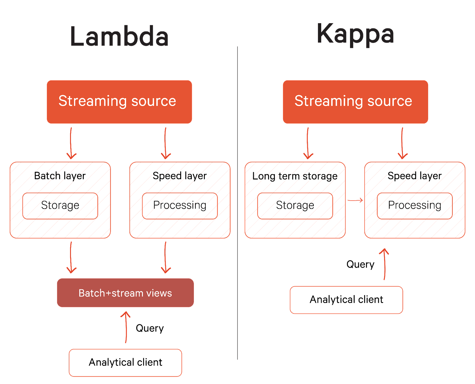
Lambda and Kappa architectures are design patterns that allow for the processing of data in real-time while also allowing for the batch processing of data for historical analysis and reporting. The Lambda architecture consists of three layers:
- The batch layer processes data in batches
- The speed layer processes data in real-time for tasks such as anomaly detection and real-time analytics.
- The serving layer serves data to applications and users, typically using a caching layer such as Apache Spark or a content delivery network (CDN).
As you would imagine, the operational complexity of Lambda Architecture requires maintaining two systems and ensuring a synchronized code base for two layers. That’s why Jay Kreps proposed a new model that completely removes the batch layer and processes all the data through streaming. This new data processing model, also known as Kappa, works on the principle of an immutable data stream, i.e., rather than point-in-time representations of databases or files, it stores logs of events.
Data consumption
Data consumption refers to analyzing and utilizing data to extract insights and support business decisions. Here's a classification of data consumption in DLM.
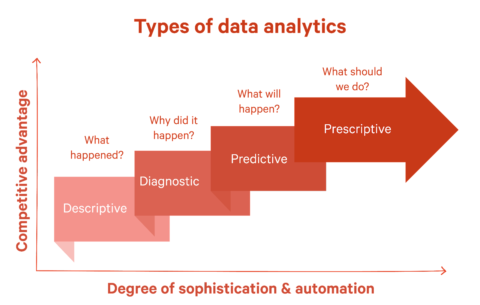
Descriptive analytics
This type of analysis helps understand what happened in the past. It involves summarizing, aggregating, and describing raw data to provide insights into historical trends, patterns, and relationships. Examples include sales reports, website traffic analytics, and customer demographics.
Diagnostic analytics
Focused on identifying why something happened, diagnostic analytics goes beyond descriptive analytics by adding more context and exploring causal relationships. Techniques used include drill-down analysis, data mining, and statistical modeling. Examples include detecting fraud, diagnosing system failures, or analyzing customer churn.
Predictive analytics
As the name suggests, predictive analytics is about forecasting what may happen. Organizations can identify potential risks, opportunities, and trends by leveraging statistical models, machine learning algorithms, and data mining techniques. Examples include credit risk assessment, demand forecasting, and personalized marketing campaigns.
Prescriptive analytics
Taking it a step further, prescriptive analytics aims to recommend the best course of action based on available data and constraints. This type of analysis uses advanced algorithms, optimization techniques, and decision science to suggest the most effective strategies, resource allocations, or process improvements. Examples include inventory management, supply chain optimization, and portfolio management.
Data archiving and deletion
Data archiving and deletion are the last stages in data lifecycle management. Archiving stores data that is no longer actively used or required for immediate access but still needs to be retained for future reference or regulatory purposes. Some standard techniques used in data archiving include:
- Data compression—reduction in the number of bits required to store data.
- Data deduplication—removal of duplicate data copies
- Data classification—based on importance and access frequency can help organizations identify which data should be archived and how it should be stored.
- Data indexing—creating indexes of archived data helps organizations quickly locate and retrieve specific data when needed.
Data validation before archiving helps ensure data integrity and accuracy. These techniques help to reduce storage costs and improve data management efficiency.
The opposite of data archival is data deletion, which securely removes data from a system or storage media, rendering it unrecoverable. Some standard techniques used in data deletion include:
- Data retention policies: Establishing policies for data retention can help organizations determine when data should be deleted and how it should be disposed of.
- Data backup and recovery: Ensuring backups are available and restorable can help organizations recover from accidental deletions or data loss.
- Auditing and monitoring: Monitoring and auditing data deletion activities can help organizations detect and respond to potential security risks or compliance violations.
Best practices in data lifecycle management
Best practices in data lifecycle management is essential for organizations that rely on large datasets to make informed decisions. These practices help ensure scalability, performance, cost savings, data quality, compliance, flexibility, reduced downtime, better collaboration, competitive advantage, and improved customer satisfaction.
Data ingestion
When ingesting, try partitioning the data into smaller subsets and process each subset in parallel. This can be done using data clustering, strata-based, or random sampling.
Use load balancing techniques to distribute the workload evenly across multiple nodes in the cluster. This ensures that no single node is overwhelmed with work and becomes a bottleneck.
Use schema-on-read to avoid imposing unnecessary structure on your data during ingestion. Instead, use flexible data formats like JSON or CSV and let the data be self-describing. This allows you to handle unexpected data format changes and new data sources more efficiently.
Data processing
Processing data out-of-order minimizes dependencies between tasks and maximizes parallelism. This can be useful when processing large datasets where some tasks may take longer than others.
Optimize memory usage to avoid bottlenecks that can slow down parallel processing. Techniques such as data compression, cache optimization, and memory pooling can help with this.
Another best practice in big data processing is to process data in place so the data is processed directly on the node where it is stored rather than moving it to a separate processing node.
Data consumption
Separating cluster resources is a best practice in big data consumption, where different parts of the data processing pipeline are processed on separate clusters or nodes.
Continuously monitor and tune the big data processing system to identify performance bottlenecks and optimize resource utilization. This includes monitoring CPU, memory, disk I/O, and network usage and adjusting parameters such as batch size, number of nodes, and data partitioning scheme.
[CTA_MODULE]
Conclusion
As technologies become more abstract and do more heavy lifting, we can think and act on a higher level. Data lifecycle management allows us to look at the bigger picture and collect, store, and process data to derive the maximum value.
Based on requirements, we can implement engineering principles from the start of the lifecycle to the end to gain insights into business intelligence and transformation while meeting all regulatory requirements.
[CTA_MODULE]